Coffee Space

Basics

This will be telling most people how to suck eggs - and for that I’m sorry. Feel free to skip through to a section better for yourself.

For those still reading, a genetic algorithm in it the simplest form is just an algorithm based on Darwin’s evolution - survival of the fittest.

This is implemented in the code like so:

0001 /* Generate fitness levels (we don't want to keep doing this) */
0002 long[] curFit = processFitness();
0003 /* Select best based on fitness */
0004 SVG[] curBest = processBest(curFit);
0005 /* Breed the best partners */
0006 breedPopulation(curBest);
0007 /* Mutate them using the mutation rate */
0008 curPolys = (int)(polys * ((double)curGen / (double)runs)) + 1;
0009 mutatePopulation();

Here you can see the important steps in this algorithm:

1. Evaluate – This is encapsulated by processFitness() and processBest(). This takes the population and generates each of their fitness values in curFit. The reason for separating the evaluation process in our implementation is that generating fitness values is really expensive.
2. Breed – This consists of the breedPopulation() function and it takes the list of best performers curFit and re-populates the population with their off-spring.
3. Mutate – Add some randomness into the genome of the population, allowing for “exploration” of the search space.

We stop doing this when the total error goes down to 0.1% or we have run out of computing time.

That’s really it! The exciting stuff is really how each of these parts is implemented.

Fitness Function

This is the first step - we need to figure out how each member of the population performs. For this implementation we convert the SVG into a bitmap image and then compare that to the original image. The larger the pixel error, the larger the number.

We do the euclidean distance of the RGB values, such that: $error = \sum_{r,g,b}^{w \cdot h}\log{\sqrt{\Delta r^2 + \Delta g^2 + \Delta b^2}}$. We calculate the maximum error as $\log{\sqrt{3 \times 256^2}} \cdot w \cdot h$. The reason for using log-error is to not over-weight large areas and to not over-weight small pixel changes.

Next we need to select a subset of the population for breeding which in the implementation uses a very basic search algorithm. It’s not particularly efficient, but compared to our other loops it’s very fast.

Breeding Function

The breeding implementation is again pretty straight forwards, we randomly select two parents from our best list (ensuring we do not select the same parent twice) and they get down and dirty. We select a random mid-point in their internal polygon layers and we take some number of polygons from one parent, and one number of polygons from another.

We then insert the child into the population and continue until we re-fill the population list.

Mutation Function

Next in the code we mutate the population, to allow the search space to be explored and to break out of local min/max optimizations.

In our implementation, we mutate two random layers and the latest layer. Why these? The latest layer will likely require the most adjust, therefore we want to concentrate our mutation efforts here. Meanwhile, we still want to be able to perform mutations to other layers to better optimize how the layers work together. Unfortunately, by mutating all of the layers together at the same time, we aren’t able to observe the independent mutations effectively and ultimately we end up with a near-random result. We therefore have to limit the amount of experimentation done in each mutation.

Shortcuts

We make a few other shortcuts that slightly speed up the implementation and generally make the result better.

1. As mentioned previously, we periodically add layers, allowing us to ‘settle’ each layer and generally find a good location for each added polygon.
2. We reduce the mutation for existing layers, meaning that they don’t move to far once we have found some nice-ish location for them.
3. The colour is calculated by centroid pixel - meaning that we don’t spend signifcant processing power picking a colour. This is also a hinderance, as it means the centroid therefore must be at a location that offers a nice colour for the entire polygon.

Results

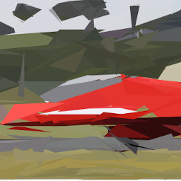
“Okay, enough of this, show me the goodies!” Sure thing! The following is the original image:

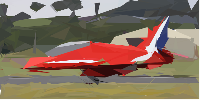
And for the output, it uses 300 polygons and took 15 minutes or so on a single core:

Bare in mind that this operated on a downsampled version and then was upsampled. I think artistically the results are actually pretty interesting for a few minutes of work. If you process for longer and add more polygons, it simply gets better and better output.

The SVG is here (but may not display well depending on your browser):

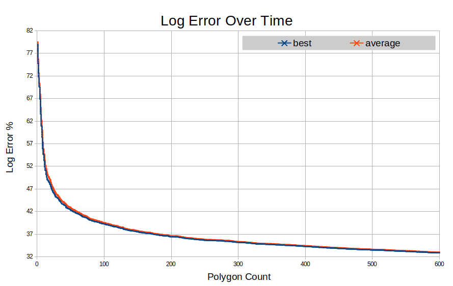
Next we have a graph displaying the error reduction over time for 600 polygons:

Note that it’s very similar to that of what you might see from something like a neural network. As you can see, clearly you get diminishing returns as you continue to add polygons. The average error sits always just above the best.

Future Work

For this project, I have a few things I would like to try:

• Multi-thread - We should be able to get massive speed-ups by enabling multiple cores.
• Pre-place polygons - This should massively reduce the time to finding a solution - we spend significant time figuring out the fact that we should probably cover holes and covering other polygons is pretty wasteful.