Coffee Space – Coffee Space

Modulo Bias

Update: Re-ran with a 6th algorithm, results and discussion reflect the performance of this.

I was reading this article by Kudelski Security Research from 2020 about modulo bias, and I found it quite interesting. As the article suggests, modulo bias is a common security issue with security reviews, and I suspect I have also seen it appear in my experiments too.

The basic idea is that you have some random variable $x$ and perform a modulo operation to limit it to the range of $y$ . We assume $x \geq 0$ and $y > 0$ , and calculate the bounded random value with $x \bmod y$ .

In these experiments we will be working on small random values where $x \leq 255$ .

Repeating Results

First things first, I want to replicate the results the author of the article generated. As in the experiments in the article, we will be be displaying the results for $y = 107$ .

These programs are run using:

0001 $ python3 <program_name> <y_value>

Random Distribution

The idea of this is just to show we produce random numbers correctly.

0002 import pandas
0003 import os
0004 import time
0005 import sys
0006 import matplotlib.pyplot as p
0007 
0008 alg = "1-bias"
0009 mod = int(sys.argv[1])
0010 
0011 start = time.time()
0012 s = pandas.DataFrame({'value':list(os.urandom(1000000))})
0013 end = time.time()
0014 
0015 s['value'].value_counts().sort_index().plot(figsize=(20,5),kind='bar')
0016 p.savefig(alg + "-" + str(mod) + ".png")
0017 
0018 print(alg, mod, (end-start) * 10**3, s.std(axis = 0, skipna = True).value)

As you can see I made some changes to the Python code to actually produce the results and give you an idea of how we will also represent the other algorithms. Note that we are also printing some other information - this will be important later.

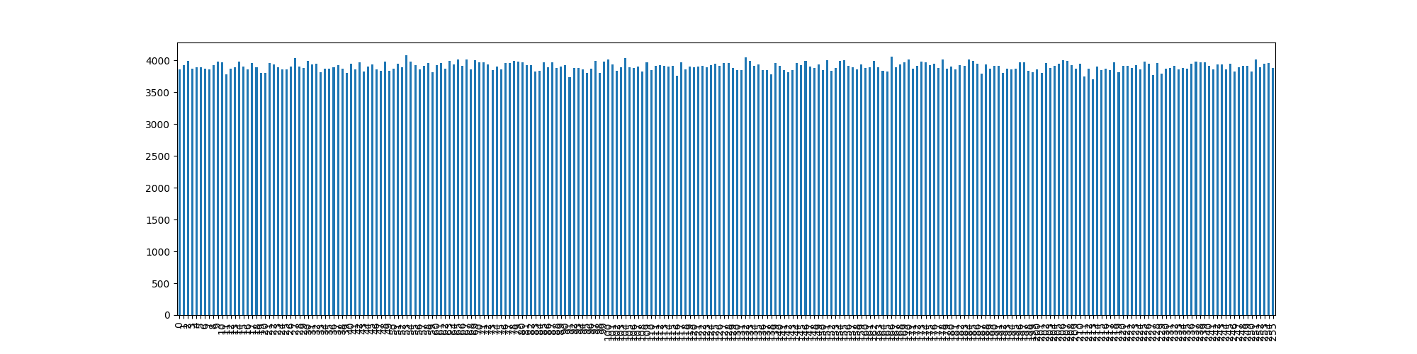
Thankfully, the local system does produce random numbers correctly. This may sound sarcastic, but Intel’s RDRAND contained a bug that meant it had to be run multiple times to produce an actually random number. AMD’s RDRAND also contained a bug meaning it would return a default value instead of a random number.

Modulo Bias

This program is for showing the bias visually.

0019 import pandas
0020 import os
0021 import time
0022 import sys
0023 import matplotlib.pyplot as p
0024 
0025 alg = "2-bias"
0026 mod = int(sys.argv[1])
0027 
0028 start = time.time()
0029 s = pandas.DataFrame({'value':[x%mod for x in os.urandom(1000000)]})
0030 end = time.time()
0031 
0032 s['value'].value_counts().sort_index().plot(figsize=(20,5),kind='bar')
0033 p.savefig(alg + "-" + str(mod) + ".png")
0034 
0035 print(alg, mod, (end-start) * 10**3, s.std(axis = 0, skipna = True).value)

As you can see, we have now introduced a bias into the output despite the input randomness being pretty good.

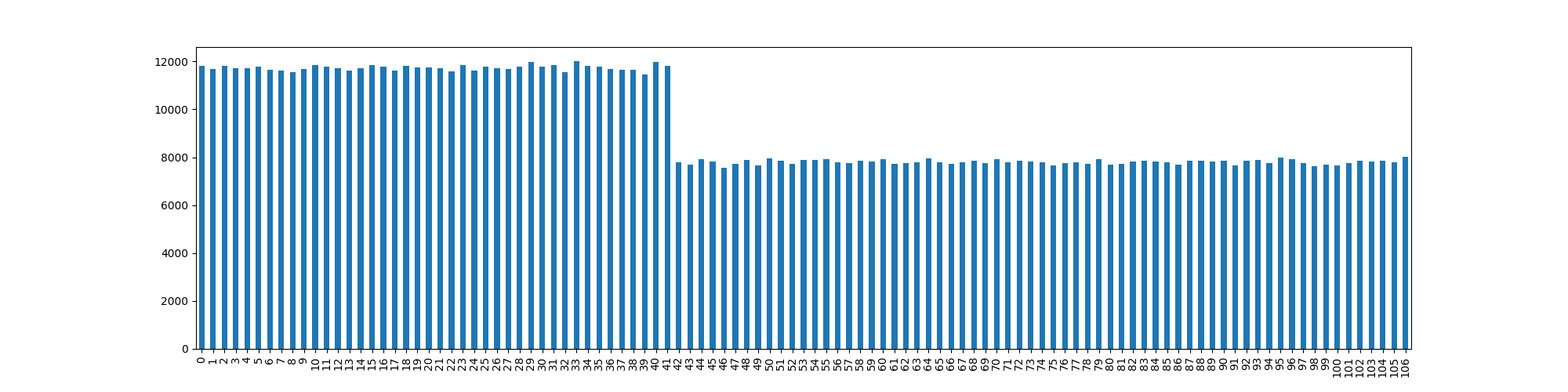
So, let’s look at how we can deal with this!

Rejection

The most obvious solution is to test the received random number and request a new one if it doesn’t meet our criteria.

0036 import pandas
0037 import os
0038 import time
0039 import sys
0040 import matplotlib.pyplot as p
0041 
0042 alg = "3-reject"
0043 mod = int(sys.argv[1])
0044 
0045 values = []
0046 start = time.time()
0047 while(len(values)<=1000000):
0048     x = int.from_bytes(os.urandom(1), byteorder='little')
0049     if x < mod:
0050         values.append(x)
0051 s = pandas.DataFrame({'value':values})
0052 end = time.time()
0053 
0054 s['value'].value_counts().sort_index().plot(figsize=(20,5),kind='bar')
0055 p.savefig(alg + "-" + str(mod) + ".png")
0056 
0057 print(alg, mod, (end-start) * 10**3, s.std(axis = 0, skipna = True).value)

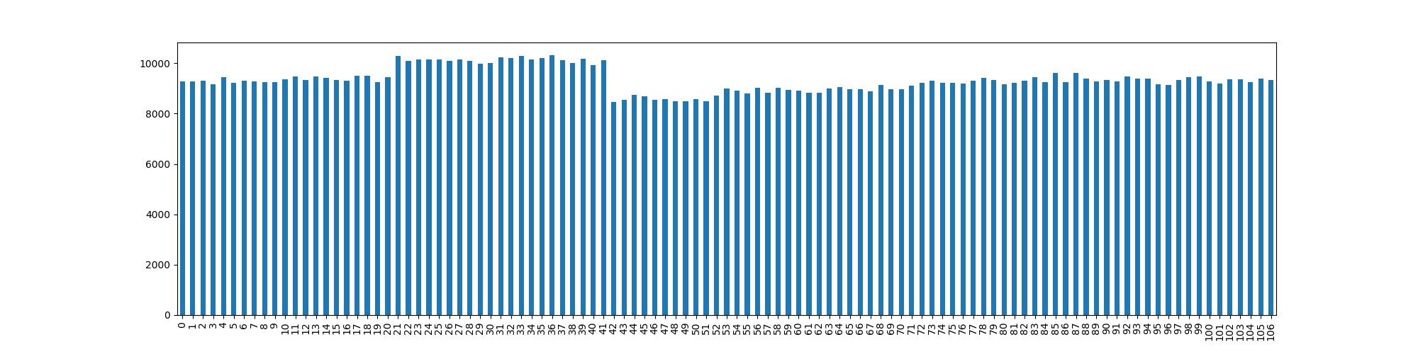
As you can see, this works really quite well! The only problem is that for low values of $y$ , it can take a long time to randomly produce a value that meets the requirement. For example, for $y = 1$ , probability it $p(y = 1) = \frac{1}{256}$ . We will plot the runtime shortly.

Rejection & Reduction

This method overcomes the issues of the previous low values of $y$ , by increasing the search space to be a multiple of $y$ . This in turn reduces the amount of rejection done without compromising the random output, increasing the running speed greatly.

0058 import pandas
0059 import os
0060 import time
0061 import sys
0062 import matplotlib.pyplot as p
0063 
0064 alg = "4-reject-reduce"
0065 mod = int(sys.argv[1])
0066 mul = mod
0067 while mul + mod < 255 :
0068   mul += mod
0069 
0070 values = []
0071 start = time.time()
0072 while(len(values)<=1000000):
0073     x = int.from_bytes(os.urandom(1), byteorder='little')
0074     if x < mul:
0075         values.append(x % mod)
0076 s = pandas.DataFrame({'value':values})
0077 end = time.time()
0078 
0079 s['value'].value_counts().sort_index().plot(figsize=(20,5),kind='bar')
0080 p.savefig(alg + ".png")
0081 
0082 print(alg, mod, (end-start) * 10**3, s.std(axis = 0, skipna = True).value)

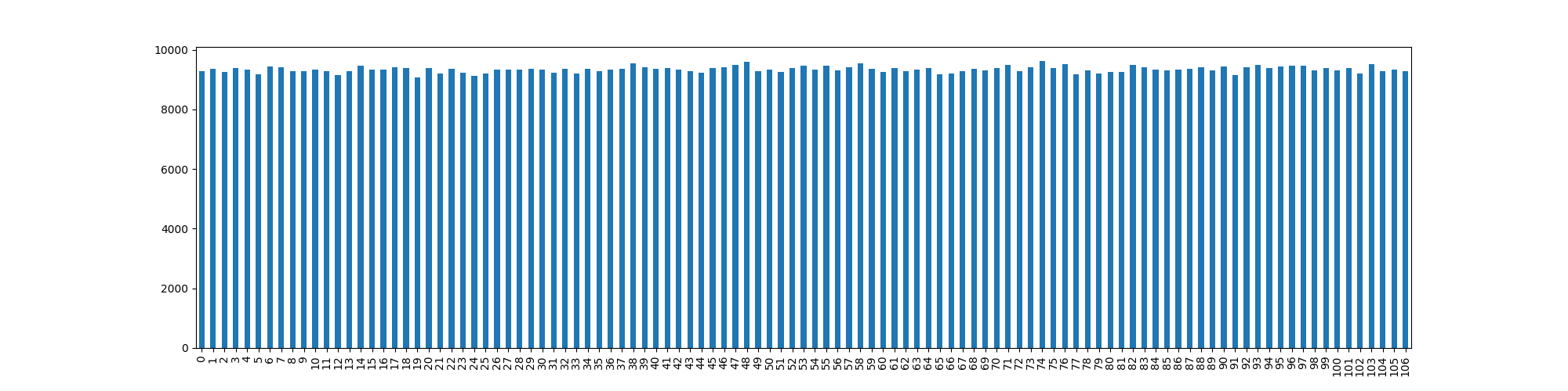
And as we can see, the results are quite nice.

Partial Rejection

The problem with rejection & reduction is that you cannot be sure it ever actually completes. Whilst it would be incredibly unlikely, it could theoretically run indefinitely. What we need is a constant-time algorithm.

This is my initial attempt at creating such. We store the previous result and XOR it with our random variable $x$ if $x$ is not within bounds. This of course means there is still a bias, but the point is that there is less of a bias.

0083 import pandas
0084 import os
0085 import time
0086 import sys
0087 import matplotlib.pyplot as p
0088 
0089 alg = "5-constant"
0090 mod = int(sys.argv[1])
0091 mul = mod
0092 while mul + mod < 255 :
0093   mul += mod
0094 
0095 values = []
0096 y = 0
0097 start = time.time()
0098 while(len(values) <= 1000000):
0099   x = int.from_bytes(os.urandom(1), byteorder = 'little')
0100   if x >= mul :
0101     x ^= y
0102   y = x % mod
0103   values.append(y)
0104 s = pandas.DataFrame({'value': values})
0105 end = time.time()
0106 
0107 s['value'].value_counts().sort_index().plot(figsize = (20, 5), kind = 'bar')
0108 p.savefig(alg + ".png")
0109 
0110 print(alg, mod, (end-start) * 10**3, s.std(axis = 0, skipna = True).value)

As we can see, the distribution is not quite as nice as either of the rejection algorithms:

But what we should gain is constant running time.

Partial Rejection v2

This is similar to the previous algorithm, except instead of XOR, we minus the previous value instead. We know that the previous value was likely less than the modulo value, and in the case that we see the generated random value $x$ is greater than the modulo value, we can minus the previous value and have a result within range.

0111 import pandas
0112 import os
0113 import time
0114 import sys
0115 import matplotlib.pyplot as p
0116 
0117 alg = "6-constant"
0118 mod = int(sys.argv[1])
0119 mul = mod
0120 while mul + mod < 255 :
0121   mul += mod
0122 
0123 values = []
0124 y = 0
0125 start = time.time()
0126 while(len(values) <= 1000000):
0127   x = int.from_bytes(os.urandom(1), byteorder = 'little')
0128   if x >= mul :
0129     # NOTE: y was likely successful in the last spin, so y < mul likely holds
0130     #       true. We know that x >= mul, so x - y should in most cases yield a
0131     #       result < mul.
0132     x -= y
0133   y = x % mod
0134   values.append(y)
0135 s = pandas.DataFrame({'value': values})
0136 end = time.time()
0137 
0138 s['value'].value_counts().sort_index().plot(figsize = (20, 5), kind = 'bar')
0139 p.savefig(alg + ".png")
0140 
0141 print(alg, mod, (end-start) * 10**3, s.std(axis = 0, skipna = True).value)

As you can see, we get a very nice distribution at this range that runs in constant time, that appears to be without significant bias:

Obviously more comprehensive testing required…

Comparison

Each of these algorithms was run for 10 runs at each modulo value, where $0 < y <= 255$ . This was run over several days, switching between algorithms (as there is currently a large day-night temperature differential which would affect CPU clock speed).

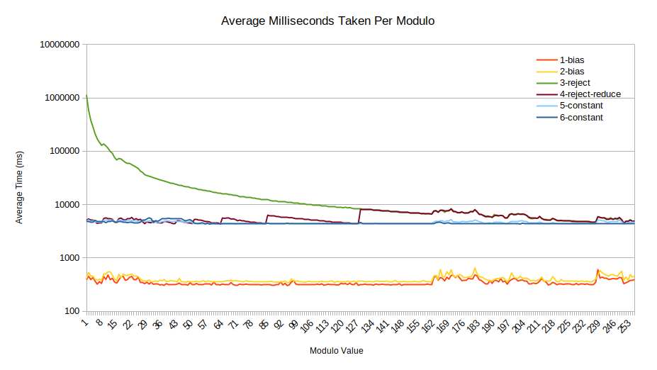
The run time for 1-bias and 2-bias are simply there for comparison. As they do not operate on the Pandas DataFrame data structure they are awarded some speed-up. Most important of note for these values is that they run near constant time.

For 3-reject we see that as expected, for lower modulo values it can take significant time to happen upon a value that occurs within bounds. For this reason we had to display the values on a logarithmic scale, as it took on average in excess of 1,000 seconds (greater than 16 minutes) per experiment. As the modulo value increases, the probability of rejection decreases, and so does the time required.

When looking at 4-reject-reduce we see a largely reduced run time, although we see a “stairs” pattern. These represent increased rejection values for given values of $y$ . In some systems this may provide probabilistic information regarding random values chosen, or the state of a pseudo random number generator (PRNG).

With 5-constant the goal was to generate random values with near constant time, which appears to have been achieved ¹. It would be difficult for a malicious actor to perform a timing-based attack based on the delay generated here.

Lastly the 6-constant algorithm is a lot more reliable for constant time work, offering the flattest line we see yet.

For completeness we see 1-bias, with a perfect standard deviation as it doesn’t limit the values within bounds. For the other algorithms, we see the deviation increase as the modulo value $y$ increases, as expected. 3-reject is our ‘perfect’ line, as it excepts nothing but truly random values within the provided bounds, at the cost of time. Equally, 4-reject-reduce simply is an iteration that reduces the number of rejections performed.

As expected, 2-bias deviates greatly, showing the bias of the output depends on the modulo value of $y$ . The algorithm 5-constant deviates somewhat, but not significantly, when compared to the deviation posed with the problematic 2-bias implementation.

The 6-constant algorithm of the other hand overcomes the issues of the 5-constant algorithm by selecting random values within the proper range, rather than trying to generate a new random value. As such the deviation is a lot tighter and appears to be cryptographically appropriate.

Discussion

As you can see in the results graphs, the modulo bias problem is quite significant. I present an algorithm of near constant time running that mostly eliminates the modulo bias problem. This may be useful for systems that need to generate many bounded random numbers with the same modulo value $y$ .

One way in which this could be used is by checking whether the previously generated random number had the same modulo, and picking a generation technique based on this fact:

0142 prev_mod = 0
0143 def gen_rand(upper_bound = 255) :
0144   x = 0
0145   if upper_bound > 0 :
0146     if prev_mod == upper_bound :
0147       x = .. # Run constant algorithm
0148     else :
0149       x = .. # Run reject and reduction
0150   prev_mod = upper_bound
0151   return x

I believe there may still be better strategies available for generating bounded random numbers that do not rely on repeated modulo values. In the future I may investigate other strategies, perhaps even looking to implement them in standard libraries for a proper comparison.