

Recently, I found myself wondering about writing a smaller, bare-bones operating system for the pure challenge of the task. Writing bloat software is one thing, but to write a lean thing of beauty is quite another.
There are several attractions to writing a small OS:
I am also looking into writing a book on the subject, something that people can interact with and should be a relatively small project. I feel as if most people want the experience, but don’t want to be engulfed by the art of writing an OS. I think writing a small, self-contained OS is ideal.
I have already written the Sax Operating System, with a bootloader/kernel bootloader in 512 bytes and have have come against, what I considered at the time, to be a pretty hard limit of how many features can be supported is such a small space.
This was until an idea occurred, which is where we are going with this article.
As any good scientist would, we need to analyse the data we have. We’re going to look at compressing some data we already have, in this case files from the older operating system mentioned previously. We’re going to be using the following files:
KERN Binary, AssemblyEDIT Binary, AssemblyRUN Binary, AssemblySPCE Binary, AssemblySYS Binary, AssemblyThese have been chosen as popular features from the old OS, hopefully being representative of the code we wish to write for the new OS.
The following Java code is used to analyse the binary data:
0001 import java.io.File;
0002 import java.io.FileInputStream;
0003 import java.io.IOException;
0004
0005 /**
0006  * Main.java
0007  *
0008  * This class represents the entire program, responsible for quickly analysing
0009  * binary blob data.
0010  **/
0011 public class Main{
0012   private static final String help =
0013     "\n[OPT] [FILE]..[FILE]" +
0014     "\n" +
0015     "\n  OPTions" +
0016     "\n" +
0017     "\n    -h --help       Display this help" +
0018     "\n    -v --version    Display program version" +
0019     "\n" +
0020     "\n  FILE" +
0021     "\n" +
0022     "\n    The binary file/s to be checked.";
0023   private static final String version = "v0.0.1";
0024
0025   /**
0026    * main()
0027    *
0028    * Initialise the main program here and parse arguments to the Main object.
0029    *
0030    * @param args The arguments to the program.
0031    **/
0032   public static void main(String[] args){
0033     new Main(args);
0034   }
0035
0036   /**
0037    * Main()
0038    *
0039    * Responsible for processing the command line arguments and processing, if
0040    * required.
0041    *
0042    * @param args The arguments to the program.
0043    **/
0044   public Main(String[] args){
0045     /* Initialise variables */
0046     String[] files = null;
0047     int size = 512;
0048     /* Process command line arguments */
0049     for(int x = 0; x < args.length; x++){
0050       switch(args[x]){
0051         case "-h" :
0052         case "--help" :
0053           exit(help);
0054           break;
0055         case "-s" :
0056         case "--size" :
0057           try{
0058             size = Integer.parseInt(args[++x]);
0059           }catch(NumberFormatException e){
0060             exit(help);
0061           }
0062           break;
0063         case "-v" :
0064         case "--version" :
0065           exit(version);
0066           break;
0067         default :
0068           if(files == null){
0069             files = new String[args.length - x];
0070           }
0071           files[args.length - x - 1] = args[x];
0072           break;
0073       }
0074     }
0075     /* Make sure there is a file to process */
0076     if(files != null){
0077       /* Create the buffer */
0078       byte[] buffer = new byte[size * files.length];
0079       /* Iterate over the files */
0080       for(int x = 0; x < files.length; x++){
0081         File f = new File(files[x]);
0082         /* Make sure the file exists */
0083         if(!f.isFile()){
0084           exit(help);
0085         }
0086         /* Read the file */
0087         try{
0088           FileInputStream fis = new FileInputStream(f);
0089           fis.read(buffer, size * x, size);
0090           fis.close();
0091         }catch(IOException e){
0092           exit(help);
0093         }
0094       }
0095       /* Analyse */
0096       System.out.println("# analyse1Pairs #");
0097       analyseNPairs(buffer, 1);
0098       System.out.println("# analyse2Pairs #");
0099       analyseNPairs(buffer, 2);
0100       System.out.println("# analyse3Pairs #");
0101       analyseNPairs(buffer, 3);
0102       System.out.println("# duplicate2Pairs #");
0103       duplicateNPairs(buffer, 2);
0104       System.out.println("# duplicate3Pairs #");
0105       duplicateNPairs(buffer, 3);
0106       System.out.println("# duplicate4Pairs #");
0107       duplicateNPairs(buffer, 4);
0108       System.out.println("# nSpacing #");
0109       nSpacing(buffer);
0110     }else{
0111       exit(help);
0112     }
0113   }
0114
0115   /**
0116    * analyseNPairs()
0117    *
0118    * Analyse N pairs of bytes in the data stream.
0119    *
0120    * @param data The data to be checked.
0121    * @param n The number of pairs to be checked, where N is less than or equal
0122    * to three.
0123    **/
0124   private void analyseNPairs(byte[] data, int n){
0125     /* Initialise the frequency array */
0126     int[] freq = new int[(int)(Math.pow(256, n))];
0127     for(int x = 0; x < freq.length; x++){
0128       freq[x] = 0;
0129     }
0130     /* Iterate over the pairs, increase the frequency */
0131     for(int x = 0; x < data.length - n + 1; x++){
0132       /* Calculate the index value */
0133       int index = 0;
0134       for(int y = 0; y < n; y++){
0135         int t = (int)(data[x + (n - y - 1)]);
0136         index += Math.pow(256, y) * (t < 0 ? 127 - t : t);
0137       }
0138       /* Increase the frequency */
0139       ++freq[index];
0140     }
0141     /* Output the results */
0142     for(int x = 0; x < freq.length; x++){
0143       /* NOTE: Only print if a result greater than zero. */
0144       if(freq[x] > 0){
0145         System.out.println(x + "\t" + freq[x]);
0146       }
0147     }
0148   }
0149
0150   /**
0151    * duplicateNPairs()
0152    *
0153    * Analyse N duplicate pairs of bytes in the data stream.
0154    *
0155    * @param data The data to be checked.
0156    * @param n The number of duplicate pairs to be checked.
0157    **/
0158   private void duplicateNPairs(byte[] data, int n){
0159     /* Initialise the frequency array */
0160     int[] freq = new int[256];
0161     for(int x = 0; x < freq.length; x++){
0162       freq[x] = 0;
0163     }
0164     /* Iterate over the pairs, increase the frequency */
0165     for(int x = 0; x < data.length - n + 1; x++){
0166       /* Calculate the index value */
0167       boolean equal = true;
0168       for(int y = 1; y < n; y++){
0169         equal &= data[x] == data[x + y];
0170       }
0171       /* Check whether values are equal */
0172       if(equal){
0173         /* Increase the frequency */
0174         ++freq[((int)data[x] < 0 ? 127 - (int)data[x] : (int)data[x])];
0175       }
0176     }
0177     /* Output the results */
0178     for(int x = 0; x < freq.length; x++){
0179       /* NOTE: Only print if a result greater than zero. */
0180       if(freq[x] > 0){
0181         System.out.println(x + "\t" + freq[x]);
0182       }
0183     }
0184   }
0185
0186   /**
0187    * nSpacing()
0188    *
0189    * Analyse the frequency of which pairs can be found with N spacing.
0190    *
0191    * @param data The data to be checked.
0192    **/
0193   private void nSpacing(byte[] data){
0194     int BYTE_SIZE = 256;
0195     /* Initialise the frequency array */
0196     int[][] freq = new int[BYTE_SIZE][];
0197     for(int y = 0; y < freq.length; y++){
0198       freq[y] = new int[BYTE_SIZE];
0199       for(int x = 0; x < freq[y].length; x++){
0200         freq[y][x] = 0;
0201       }
0202     }
0203     /* Iterate over the pairs, increase the frequency */
0204     for(int o = 0; o < data.length; o++){
0205       /* Iterate over the spacing tests */
0206       for(int n = 1; n < BYTE_SIZE && n + o < data.length; n++){
0207         /* Check if current character is found after N spaces */
0208         if(data[o] == data[o + n]){
0209           ++freq[n][((int)data[o] < 0 ? 127 - (int)data[o] : (int)data[o])];
0210         }
0211       }
0212     }
0213     /* Output the results */
0214     for(int y = 0; y < freq.length; y++){
0215       for(int x = 0; x < freq[y].length; x++){
0216         /* Only print not zero results */
0217         if(freq[y][x] != 0){
0218           System.out.println(y + "\t" + x + "\t" + freq[y][x]);
0219         }
0220       }
0221     }
0222   }
0223
0224   /**
0225    * exit()
0226    *
0227    * Hard exit the program with a message.
0228    *
0229    * @param msg The message to be displayed.
0230    **/
0231   private void exit(String msg){
0232     System.out.println(msg);
0233     System.exit(0);
0234   }
0235 }
NOTE: LibreOffice graphs can be found here.
First things first, we need to find out how this binary data is distributed:
For only a little work, this is some nice results to see. Some interesting points for me:
0dFrom this, we can conclude that this is compressible data!
Here we analyse the possibility of some dictionary related lookup system, by analysing how pairs of data is distributed in our sample sets. The result is stored as a decimal, where we only keep frequencies larger than zero. This is because when originally testing the software, for some reason the Java heap doesn’t like 256 ^ 4 lookup tables, not sure why (sarcasm).
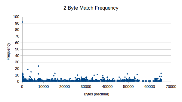
As you can see from these results, it should certainly be possible for compression on 2 byte pairs in our data, even from small 512 byte chunks.
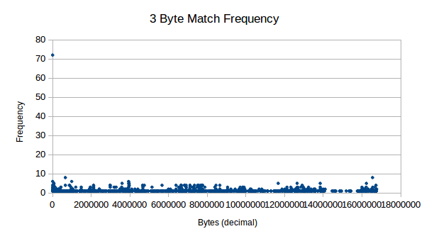
Next, we see 3 byte pairs, which also show decent levels of
frequency. These don’t seem to tend much higher than “background noise”
for all aspects other than 0.
In order for a dictionary method of compression to work, we can first make some assumptions about in order to theoretically test feasibility:
We can now calculate how much data we need to replace in order to make the process worth our time:
This can now be expressed as y = mx + c, or
y = (3 * x) - 50. In order to break even, so that
y = 0, we must calculate 50 / 3 = x, which is
17 matches. In order to save 50 bytes, comparable to the implementation
of the decompression algorithm, we must calculate where
y = 50, so that (50 + 50) / 3, which is 34
matches. In just 512 bytes, this is a push.
Of course, this doesn’t take into consideration the data required to describe the replacements, further eating into any gains we may have. In order for this system to work, there must be a high amount of overlapping dictionary mappings, otherwise the description of the replacement will cost more than the gain from the replacement.
Yet another interesting pattern (a subset pattern from the one discussed previously) in the data is where we see duplicates of data side-by-side with the same value. Consider the following results:
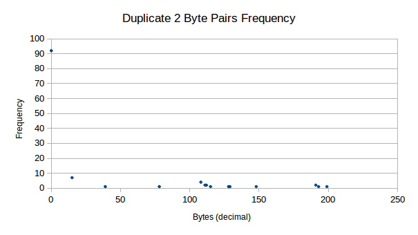
We see that firstly, we have many duplicate zeros in our data. Other
than this, there are still very strong presences of duplicate data for
other values, mainly for 15d, where we see 7 strong
counts.
There are some benefits to duplicate representation:
On the negative side, duplicates are much less likely to occur in 125
bytes. Somewhere between 46 / 285 and 92 / 285
of our data is side-by-side zeros, representing space that we can fit
more programming code in anyway. This greatly reduces the benefit of
using this method.
These tables are now too small to even produce a graph that has any advantage, so we display our raw results here:
0236 Duplicate Match_Index Frequency
0237 3         0           72
0238 3         15          6
0239 4         0           65
0240 4         15          5
Specifically, byte 15d is of interest, as this byte
seems highly compressible. Assuming this value is related to an opcode,
0x0F seems to be used for popping data from the stack Wikipedia.
This would mean that in our code, after using one pop
instruction, we are quite likely to use another - which is certainly an
interesting find.
Here we decide to look at characters that repeat after N spaces, the idea being that we can compress two bytes down into one byte that describes the current character and it’s repeat location. A example of this is below:
0241 X  = 'a'  2
0242 S  = 'a' 'b' 'c' 'a' 'd'
0243 S' =  X  'b' 'c' 'd'
So in this example, the description is that X denotes
that the character 'a' exists in the place of
X, but also in an offset of 2 characters. Used
in the example string S, we see that we are able to
compress our string to S'. In out testing, we limit the
spacing to 255 spaces, as this still easily fits in an 8 bit byte and
makes the data description smaller to work with.
Now we analyse the results:
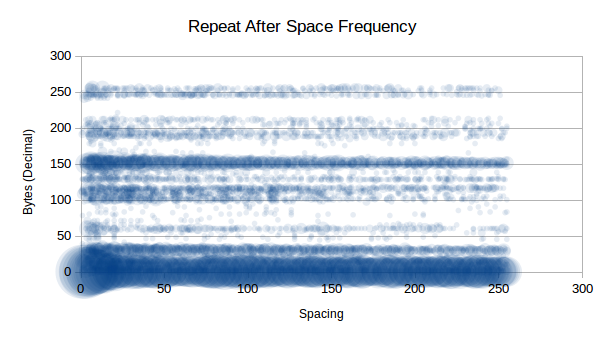
As you can see, 0d is clearly highly compressible as we
saw in previous tests, but now we see that there are some other highly
compressible data that don’t repeat immediately, such as
150d. Interestingly that is not an x86 instruction.
A list interesting (repeats 5 or more times) repeats include:
0d - No spacing1d - Possible VM call10d - New line13d - Carriage return15d - Pop instruction29d - No information32d - Space character or logical AND instruction60d - No information101d - No information116d - No information117d - No information150d - No information151d - No information156d - Push flags instruction188d - No information251d - Set interrupt flag instruction255d - Call or decrement or increment or jump
instructionLooking past the highly compressible 0d, which will be
unlikely to be in our final compression data, we the following order of
compressible data (just some):
151d at 20 spaces is compressible
20 times150d at 6 spaces is compressible
16 times29d at 13 spaces is compressible
11 times60d at 4 spaces is compressible
9 times255d at 7 spaces is compressible
7 times117d at 10 spaces is compressible
7 times32d at 7 spaces is compressible
7 timesWe potentially have 31 bytes at our disposal to represent N-spaced
repeats, so as long as the savings are greater than the cost of
representation (<INDICATOR> +
<CHAR> + <SPACING>), then we shall
see savings.
Assuming we get half of the saving mentioned in our list, that would be:
0244 (20 + 16 + 11 + 9 + 7 + 7 + 7) / 2 = 38.5 ~= 38 bytes
That 38 bytes saved, minus the representation bytes,
7 * 3 = 21, leaves us a saving off 17 bytes. Of course, the
implementation of the decompression also will have a cost, meaning we
will use more bytes than we save with any reasonably sized OS. Back to
the drawing board!
So a crazy idea I had was to implement a bubble-sort inspired compression algorithm, something that seemed on paper that may have some merit. I decided to write a program to explore the idea, so that I could approach this idea with a Scientific approach.
Here is the test program:
0245 import time
0246
0247 debug = False
0248
0249 # ordered()
0250 #
0251 # Check if the data is ordered.
0252 #
0253 # @param data The stream to be tested.
0254 # @return True if ordered, otherwise False.
0255 def ordered(data) :
0256   for x in range(0, len(data) - 1) :
0257     if data[x] > data[x + 1] :
0258       return False
0259   return True
0260
0261 # decompressed()
0262 #
0263 # Check whether the data has been decompressed.
0264 #
0265 # @param data The stream to be tested.
0266 # @return True if decompressed, otherwise False.
0267 def decompressed(data) :
0268   for x in range(0, len(data) - 1) :
0269     if data[x] == float("inf") :
0270       return False
0271   return True
0272
0273 # order()
0274 #
0275 # Orders a set of data. Functional method.
0276 #
0277 # @param data The data stream to be tested.
0278 # @return The ordered data.
0279 def comp(data) :
0280   # Initialise variables
0281   indx = 0
0282   # Infinite loop until complete
0283   while 1 :
0284     # Display what we have
0285     if debug == True :
0286       print(str(indx) + "::" + str(data))
0287     # Make sure we're not at the end
0288     if ordered(data) == True :
0289       return data
0290     # Check if we're at the end
0291     if indx >= len(data) - 1 :
0292       indx = 0
0293     # Check whether ordering required for this pair
0294     if data[indx] > data[indx + 1] :
0295       tmp = data[indx]
0296       data[indx] = data[indx + 1]
0297       data[indx + 1] = tmp
0298       data.insert(indx + 2, float("inf"))
0299     # Next check
0300     indx += 1
0301   # Should never reach here!
0302   print("ERROR!")
0303
0304 # decomp()
0305 #
0306 # Decompress the data stream. Functional method.
0307 #
0308 # @param data The data stream to be tested.
0309 # @return The unordered data.
0310 def decomp(data) :
0311   # Initialise variables
0312   indx = 0
0313   # Infinite loop until complete
0314   while 1 :
0315     # Display what we have
0316     if debug == True :
0317       print(str(indx) + "::" + str(data))
0318     # Make sure we're not at the end
0319     if decompressed(data) == True :
0320       return data
0321     # Check if we're at the end
0322     if indx <= 2 :
0323       indx = len(data) - 1
0324     # Check whether ordering required for this pair
0325     if data[indx] == float("inf") :
0326       tmp = data[indx - 1]
0327       data[indx - 1] = data[indx - 2]
0328       data[indx - 2] = tmp
0329       data.pop(indx)
0330     # Next check
0331     indx -= 1
0332   # Should never reach here!
0333   print("ERROR!")
0334
0335 tests = [
0336   [4, 2, 1, 3],
0337   [4, 3, 2, 1],
0338   [3, 4, 1, 2],
0339   [3, 2, 4, 1],
0340   [1, 2, 1, 2],
0341   [2, 1, 2, 1],
0342   [4, 2, 1, 3, 4],
0343   [4, 2, 1, 3, 4, 3],
0344   [4, 2, 1, 3, 4, 3, 2],
0345   [4, 2, 1, 3, 4, 3, 2, 1],
0346   [4, 2, 1, 3, 4, 3, 2, 1, 3],
0347   [4, 2, 1, 3, 4, 3, 2, 1, 3, 4],
0348   [4, 2, 1, 3, 4, 3, 2, 1, 3, 4, 1],
0349   [4, 2, 1, 3, 4, 3, 2, 1, 3, 4, 1, 2],
0350   [4, 2, 1, 3, 4, 3, 2, 1, 3, 4, 1, 2, 3]
0351 ]
0352
0353 print("TEST,INITIAL_SIZE,START_TIME,DEFLATED_SIZE,COMPRESSION_TIME,DECOMPRESSION_TIME,RESULT")
0354 for x in range(0, len(tests)) :
0355   output = "\"" + str(tests[x]) + "\","
0356   output += str(len(tests[x])) + ","
0357   output += str(time.time()) + ","
0358   c = comp(tests[x])
0359   output += str(len(c)) + ","
0360   output += str(time.time()) + ","
0361   d = decomp(c)
0362   output += str(time.time()) + ","
0363   if c == d :
0364     output += "EQUAL"
0365   else :
0366     output += "NOT_EQUAL"
0367   # Output the results
0368   print(output)
This produced the following results (original here):
0369 SIZE DEFLATE COMPRESS        DECOMPRESS
0370 4    15      0               0
0371 4    21      0               0
0372 4    13      0               0
0373 4    15      0               0
0374 4    6       0               0
0375 4    11      0               0
0376 5    27      0               0
0377 6    53      0               0
0378 7    116     0.0099999905    0
0379 8    289     0.0700001717    0
0380 9    574     0.6699998379    0
0381 10   1140    4.9600000381    0.0099999905
0382 11   2526    46.3900001049   0.0199999809
0383 12   5105    522.2400000095  0.129999876
0384 13   10206   5851.7400000095 0.7999999523
Now we can now take a look at the feasibility of the project and whether we are looking at a good compression method or if this is not feasible.
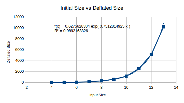
Here we are looking at initial size vs deflated size, the purpose of
this is to look at RAM usage from decompression. This doesn’t initially
look too bad, until you plug in x = 512 (512 bytes to
compress), giving you ~1x10^167… Oh my, this is a good start. We won’t
stop here, there may be some technique to compress this is RAM during
decompression - so we shan’t worry too much about this.
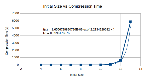
This is a show stopper - it looks as if no current computer could even compress 512 bytes using this method, in some human feasible time. By the looks of this, it could literally take a lifetime to compute the compressed data set.
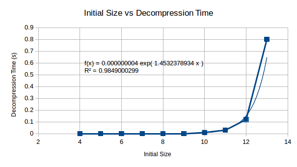
The decompression starts with small values, but appears as though it too would become an extremely time consuming process wants extended to 512 bytes worth. The following graph allows us to make a decision as to whether this will be an issue for us.
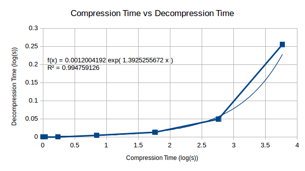
Looking at the relationship between compression and decompression, we see that compression becomes a much harder problem than decompression. This suggests that although the compression complexity is high for this algorithm, decompression will become less complex in comparison and may be computable on a reasonably well powered machine.
To conclude, there are two major problems with this compression algorithm that make it useless until solved:
It looks as though, for now, this one is off the table until a later date. This is why we test ;)
Tasks:
[X] Analyse frequency of bytes[X] Analyse frequency of 2-pair repeat bytes[X] Analyse frequency of 3-pair repeat bytes[X] Analyse duplicate frequency of 2-pair repeat
bytes[X] Analyse duplicate frequency of 3-pair repeat
bytes[X] Analyse duplicate frequency of 4-pair repeat
bytes[X] Analyse N spacing repeat frequency[ ] Research compression algorithms[~] Design compression algorithms